
Suppose we are having an exit interview with two employees: John, and James. We have two simple questions: “What are the Pros of working at Company X?” and “What are the Cons of working at Company X?” Given that one of those employees genuinely love the company, but the other one hates it. I’d imagine the interviews probably be like this:
John
Pohnson: John, what are the pros of working at Company X?
John: Pohnson, that question is simple, but I’m not sure if our one-hour meeting can fit all that I have to say about our company. Let’s talk about the top 10 in my list. First, I love because… and the list goes on.
Pohnson: John, what are the cons of working at Company X?
John: [long pause] I cannot think of any.
Then I interview James who hates Company X.
James
Pohnson: James, what do you like about our company?
James: [long pause] I cannot think of any.
Pohnson: James, what are the cons of working at this company?
James: Pohnson, that question is simple, but I’m not sure if our one-hour meeting can fit all that I have to say about our company. Let’s talk about the top 10 in my list. First, I hate because… and the list goes on.
If the case holds true, counting the number of word in each answer should give us a clue into an employee’s mind. I mean, if you like a company, you should find a lot more to talk about Pros than Cons, right? But if you don’t, you probably have a lot to say in Cons.
Let’s do exactly that. But first, we need to load goodies.
|
1 2 3 4 5 6 7 8 9 10 11 12 13 14 15 16 17 18 |
##### Load Goodies ##### library(tidyverse) library(stringr) library(stringi) library(ggrepel) ##### Create Theme for GGPLOT2 ##### theme_moma <- function(base_size = 12, base_family = "Helvetica") { theme( plot.background = element_rect(fill = "#F7F6ED"), legend.key = element_rect(fill = "#F7F6ED"), legend.background = element_rect(fill = "#F7F6ED"), panel.background = element_rect(fill = "#F7F6ED"), panel.border = element_rect(colour = "black", fill = NA, linetype = "dashed"), panel.grid.minor = element_line(colour = "#7F7F7F", linetype = "dotted"), panel.grid.major = element_line(colour = "#7F7F7F", linetype = "dotted") ) } |
I scraped the reviews by creating a separate R project for each company. So, I had to use read.csv() for each firm and combine them in this project. As the files are in a CSV format, we can use the for loop() to load them into the work environment.
|
1 2 3 4 5 6 7 8 9 10 |
##### Load Data ##### list <- data.frame(file = list.files(pattern = "*.csv")) list$name <- str_replace_all(list$file, ".csv", "") for (i in 1:nrow(list)){ filename <- as.character(list[i,1]) assign(paste(list[i,2]), read.csv(filename)) rm(filename, i) } |
As I didn’t change the scraping codes, the columns are the same. So, what we need to do is very simple: format the date, remove punctuation, and remove a placeholder row. But since Microsoft has two different date formats, I’ll just deal with its first, then initiate the for loop() .
|
1 2 3 4 5 6 7 8 9 10 11 12 13 14 15 16 17 18 19 20 21 22 |
##### MSFT Date ##### temp_1 <- msft[1:301,] temp_2 <- msft[302:6411,] temp_1$Posted_Date <- as.Date(temp_1$Posted_Date, format = "%d %b, %Y") temp_2$Posted_Date <- as.Date(temp_2$Posted_Date, format = " %b %d, %Y") msft <- rbind(temp_1,temp_2) rm(temp_1,temp_2) ##### For Loop for Processing ##### for (i in 1:nrow(list)){ name <- list[i,2] assign(list[i,2], mutate(get(list[i,2]), Summary_2 = str_replace_all(Summary, "[:punct:]", ""), Pros_2 = str_replace_all(Pros, "[:punct:]", ""), Cons_2 =str_replace_all(Cons, "[:punct:]", ""), Date = as.Date(Posted_Date, format = " %b %d, %Y"), Company = as.character(list[i,2]))) } |
Now, we are ready to combine them using rbind() .
|
1 |
aggregate <- rbind(airbnb, amzn, apple, expedia, fb, google, msft, sbux, tmobile, uber) |
Next, we remove the placeholder row, and create new variables.
|
1 2 3 4 5 6 |
aggregate <- aggregate %>% select(Pros_2, Cons_2, Date, Company) %>% filter(Pros_2 != 'xx') %>% arrange(Company, Date) %>% mutate(Pros_count = stri_count_boundaries(Pros_2), Cons_count = stri_count_boundaries(Cons_2)) |
Let’s start by creating boxplots.
|
1 2 3 4 |
ggplot(data=aggregate, aes(x = Company, y = Pros_count)) + geom_boxplot() + theme_moma() + ggtitle("Pros") |

1,200 words for FB’s Pros… whoever wrote this was sure an admirer. But what about cons?
|
1 2 3 4 |
ggplot(data=aggregate, aes(x = Company, y = Cons_count)) + geom_boxplot() + theme_moma() + ggtitle("Cons") |

Over 2,000 words for Amzn’s Cons… I sense discontents.
I think we need to make some adjustment as the outliers distorted the chart.
|
1 2 3 4 |
aggregate %>% filter(Cons_count < 100) %>% ggplot(aes(x = Company, y = Cons_count)) + geom_boxplot() + theme_moma() |
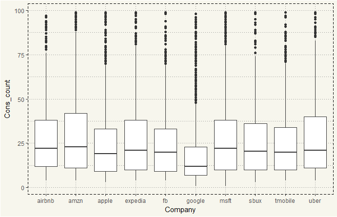
It seems like Google on average is the lowest. But we can do better than that. Let’s create summarized values and create a slope chart.
|
1 2 3 4 5 6 7 8 9 10 11 12 13 14 15 16 |
##### Columns for Slope Charts ##### aggregate_2 <- aggregate %>% group_by(Company) %>% mutate(Pros_avg = round(mean(Pros_count)), Cons_avg = round(mean(Cons_count)), Pros_median = median(Pros_count), Cons_median = median(Cons_count), avg_more = ifelse(Pros_avg > Cons_avg, "green", "red"), median_more = ifelse(Pros_median > Cons_median, "green", "red"), avg_label_pros = paste(Company, Pros_avg, sep = " "), avg_label_cons = paste(Company, Cons_avg, sep = " "), median_label_pros = paste(Company, Pros_median, sep = " "), median_label_cons = paste(Company, Cons_median, sep = " "))%>% select(-Date, -Pros_2, -Cons_2) dim(aggregate_2) |
|
1 2 |
> dim(aggregate_2) [1] 18462 13 |
That’s too many observations. Since we only need ten distinct values, let’s use distinct() .
|
1 2 3 |
aggregate_3 <- distinct(select(aggregate_2, -Pros_count, - Cons_count)) aggregate_3 |
|
1 2 3 4 5 6 7 8 9 10 11 12 13 14 15 16 |
> aggregate_3 # A tibble: 10 x 11 # Groups: Company [10] Company Pros_avg Cons_avg Pros_median Cons_median avg_more median_more avg_label_pros avg_label_cons median_label_pros <chr> <dbl> <dbl> <dbl> <dbl> <chr> <chr> <chr> <chr> <chr> 1 airbnb 41 44 26 24 red green airbnb 41 airbnb 44 airbnb 26 2 amzn 34 54 21 27 red red amzn 34 amzn 54 amzn 21 3 apple 26 38 17 20 red red apple 26 apple 38 apple 17 4 expedia 30 40 19 23 red red expedia 30 expedia 40 expedia 19 5 fb 41 32 25 21 green green fb 41 fb 32 fb 25 6 google 16 22 10 12 red red google 16 google 22 google 10 7 msft 27 39 19 23 red red msft 27 msft 39 msft 19 8 sbux 25 39 18 23 red red sbux 25 sbux 39 sbux 18 9 tmobile 23 35 16 22 red red tmobile 23 tmobile 35 tmobile 16 10 uber 44 38 30 23 green green uber 44 uber 38 uber 30 # ... with 1 more variables: median_label_cons <chr> |
Now, that’s much better. Let’s see the mean slope plot.
|
1 2 3 4 5 6 7 8 9 10 11 12 13 14 15 16 17 18 |
##### Mean Slope Plot ##### mean_slope_plot <- ggplot(aggregate_3) + geom_segment(aes(x = 1, xend = 2, y = Pros_avg, yend = Cons_avg, col = avg_more), size = .75, show.legend = FALSE) + geom_vline(xintercept=1, linetype="dashed", size=.1) + geom_vline(xintercept=2, linetype="dashed", size=.1) + scale_color_manual(labels = c("Up", "Down"), values = c("green"="#00ba38", "red"="#f8766d")) + labs(x="", y="Word Count") + xlim(.5, 2.5) + ylim(15,(1.1*(max(aggregate_3$Pros_avg, aggregate_3$Cons_avg)))) + theme_moma() mean_slope_plot <- mean_slope_plot + geom_text_repel(label=aggregate_3$avg_label_pros, y=aggregate_3$Pros_avg, x=rep(1, NROW(aggregate_3)), size=3.5) + geom_text_repel(label=aggregate_3$avg_label_cons, y=aggregate_3$Cons_avg, x=rep(2, NROW(aggregate_3)), size=3.5) + geom_text(label="Pros", x=1, y=1.1*(max(aggregate_3$Pros_avg, aggregate_3$Cons_avg)), hjust=1.2, size=5)+ geom_text(label="Cons", x=2, y=1.1*(max(aggregate_3$Pros_avg, aggregate_3$Cons_avg)), hjust=-0.1, size=5) mean_slope_plot |
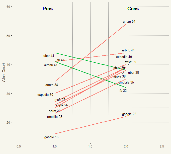
Only Uber and FB has more words in Pros than Cons. The slope of each company is about the same. Amazon has the steepest slope.
But as we have seen in the boxplot, outliers will make the mean higher than it should be. So, let’s try median.
|
1 2 3 4 5 6 7 8 9 10 11 12 13 14 15 16 17 18 |
##### Median Slope Plot ##### median_slope_plot <- ggplot(aggregate_3) + geom_segment(aes(x = 1, xend = 2, y = Pros_median, yend = Cons_median, col = median_more), size = .75, show.legend = FALSE) + geom_vline(xintercept=1, linetype="dashed", size=.1) + geom_vline(xintercept=2, linetype="dashed", size=.1) + scale_color_manual(labels = c("Up", "Down"), values = c("green"="#00ba38", "red"="#f8766d")) + # color of lines labs(x="", y="Mean GdpPerCap") + # Axis labels xlim(.5, 2.5) + ylim(5,(1.1*(max(aggregate_3$Pros_median, aggregate_3$Cons_median)))) + theme_moma() median_slope_plot <- median_slope_plot + geom_text_repel(label=aggregate_3$median_label_pros, y=aggregate_3$Pros_median, x=rep(1, NROW(aggregate_3)), size=3.5) + geom_text_repel(label=aggregate_3$median_label_cons, y=aggregate_3$Cons_median, x=rep(2, NROW(aggregate_3)), size=3.5) + geom_text(label="Pros", x=1, y=1.1*(max(aggregate_3$Pros_median, aggregate_3$Cons_median)), hjust=1.2, size=5) + geom_text(label="Cons", x=2, y=1.1*(max(aggregate_3$Pros_median, aggregate_3$Cons_median)), hjust=-0.1, size=5) median_slope_plot |
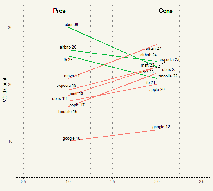
It’s just about the same. With median, AirBNB has fewer words in Cons than in Pros.
So, it seems like when the time to talk about reviewers’ employer, reviewers have more to say about Cons than Pros except Uber and Facebook.