
Let’s load goodies and create theme
|
1 2 3 4 5 6 7 8 9 10 11 12 13 14 15 16 |
##### Load Goodies ##### library(tidyverse) library(glmnet) ##### Theme ##### theme_moma <- function(base_size = 12, base_family = "Helvetica") { theme( plot.background = element_rect(fill = "#F7F6ED"), legend.key = element_rect(fill = "#F7F6ED"), legend.background = element_rect(fill = "#F7F6ED"), panel.background = element_rect(fill = "#F7F6ED"), panel.border = element_rect(colour = "black", fill = NA, linetype = "dashed"), panel.grid.minor = element_line(colour = "#7F7F7F", linetype = "dotted"), panel.grid.major = element_line(colour = "#7F7F7F", linetype = "dotted") ) } |
We will use mtcars data to demonstrate the power of Ridge regression for model selection. First, we need to prep our data and see if there is any missing value.
|
1 2 3 |
##### Data Prep ##### data <- mtcars sum(is.na(data)) |
|
1 2 |
> sum(is.na(data)) [1] 0 |
Good, there is no missing value. We will use the glmnet() function to perform Ridge Regression. Unlike lm() , glmnet() cannot take data frame. Therefore, we need two additional steps. First, we need to create a matrix.
|
1 2 |
##### Creating Data Matrix ##### predictors <- model.matrix(mpg ~ ., data)[,-1] |
Next, we separate the independent variable out.
|
1 |
y <- data$mpg |
Recall that Ridge Regression has the penalty parameter as follows:
$$\lambda\sum_{j=1}^{p}\beta_j^2$$
As we need to specify the value of \(\lambda\), we can either get the value by manually specifying the value or applying other cross-validation technique such as k-Folds or LOOCV. But before the steps, we need to divide the data into a training set and a test set.
|
1 2 3 4 5 |
##### Splitting Train and Test Sets ##### train_number <- round(0.8*nrow(data),digit=0) set.seed(999) train_index <- sample(seq_len(nrow(data)), size = train_number) test_index <- (-train_index) |
Choosing \(\underline\lambda\) Manually
As glmnet() cannot take a data frame, we will use an index to subset data. Then we fit the Ridge Regression model.
|
1 2 3 4 5 |
##### Fitting the Model ##### ridge <- glmnet(predictors[train_index,], y[train_index], alpha = 0, thresh = 1e-7) |
By default, the function will generate 100 values of \(\lambda\). We can create a loop to calculate MSE of each value.
|
1 2 3 4 5 6 7 8 9 |
##### For Loop() for MSE ##### MSE <- rep(0,100) for (i in 1:100){ ridge.pred <- predict(ridge, s=ridge$lambda[i], newx = predictors[test_index,]) print(ridge$lambda[i]) MSE[i] <- mean((ridge.pred - y[test_index])^2) } |
Then we visualize.
|
1 2 3 4 5 6 7 8 9 10 11 12 13 14 15 16 17 18 19 20 21 22 |
##### Creating Data for Visualization ##### lambda_mse <- data.frame(lambda = ridge$lambda, MSE = MSE, index = c(1:100)) image_mse <- ggplot(lambda_mse,aes(x = index, y = MSE)) + geom_line() + geom_point() + theme_moma() + geom_point(data = subset(lambda_mse, MSE < 6.2), aes(x = index, y = MSE), size = 2, col = 'red') + geom_vline(xintercept = 78, linetype = "dashed", col = 'red') image_lambda <- ggplot(lambda_mse,aes(x = index, y = lambda)) + geom_line() + geom_point() + theme_moma() + geom_point(data = subset(lambda_mse, MSE < 6.2), aes(x = index, y = MSE), size = 2, col = 'red') + geom_vline(xintercept = 78, linetype = "dashed", col = 'red') grid.arrange(image_mse, image_lambda, nrow = 1) |
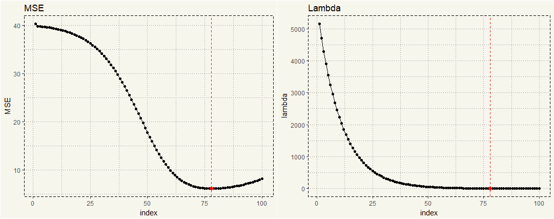
Now we can see that the lowest MSE is somewhere between 75 and 78. Dplyr can give us a better view.
|
1 2 3 4 |
##### Min Value ##### lambda_mse %>% arrange(MSE) %>% head() |
|
1 2 3 4 5 6 7 8 9 10 |
> lambda_mse %>% + arrange(MSE) %>% + head() lambda MSE index 1 3.995793 6.196998 78 2 3.640818 6.201139 79 3 4.385378 6.204092 77 4 3.317377 6.215569 80 5 4.812947 6.223577 76 6 3.022671 6.236978 81 |
We can get coefficients through coef() .
|
1 2 |
##### Coefficients ##### coef(ridge)[,78] |
|
1 2 3 4 5 |
> coef(ridge)[,78] (Intercept) cyl disp hp drat wt qsec vs 18.639909198 -0.351549475 -0.006064874 -0.010942877 1.157517083 -1.281056096 0.293076129 0.572151466 am gear carb 1.569683802 0.350575028 -0.411282309 |
But we need to manually calculate L2 norm.
|
1 2 |
##### L2 Norm ##### sqrt(sum(coef(ridge)[-1,78]^2)) |
|
1 2 |
> sqrt(sum(coef(ridge)[-1,78]^2)) [1] 2.504777 |
Choosing \(\underline\lambda\) Through k-CV
Glmnet library has cv.glmnet() function that can automatically perform a k-CV.
|
1 2 3 4 5 6 |
##### CV ##### set.seed(999) kcv <- cv.glmnet(predictors[train_index,], y[train_index],alpha=0) ##### Names ##### names(kcv) |
|
1 2 3 |
> names(kcv) [1] "lambda" "cvm" "cvsd" "cvup" "cvlo" "nzero" "name" "glmnet.fit" [9] "lambda.min" "lambda.1se" |
The \(\lambda\) with lowest associated MSE is stored in ‘lambda.min’ that we can access through subsetting.
|
1 2 3 |
##### Accessing Lambda ##### bestlambda <- kcv$lambda.min bestlambda |
|
1 2 |
> bestlambda [1] 1.436013 |
We then use the \(\lambda\) in the predict() .
|
1 2 3 4 5 |
##### K-CV in Action ##### kcv_predict <- predict(ridge, s = bestlambda, newx = predictors[test_index,]) mean((kcv_predict - y[test_index])^2) |
|
1 2 3 4 5 |
> kcv_predict <- predict(ridge, + s = bestlambda, + newx = predictors[test_index,]) > mean((kcv_predict - y[test_index])^2) [1] 6.711412 |
Two methods give slightly different lambda as the first method trained on the entire dataset, while the second method is k-CV. Now, is MSE value of 6 considered low? Let’s compare with plain lm() .
|
1 2 3 4 5 |
##### Just LM ##### lm <- lm(mpg ~ ., data[train_index,]) lm_predict <- predict(lm, newdata = data[test_index,]) mean((lm_predict - y[test_index])^2) |
|
1 2 |
> mean((lm_predict - y[test_index])^2) [1] 18.97969 |
Yep, MSE value of 6 is indeed low and can be considered an improvement.